01 — On Listening and Duets
Hearing Performance, Chaotic Dynamics, and Computational Auditory Scene Analysis
Erick Oduniyi — originally with Myunghyun Oh
Motivation
This project started from a deep appreciation for mathematics, music, and sound. The question at its core: how do we hear a duet?
When two musicians play together, the sound waves arriving at your ears are a single, tangled pressure signal. Yet you effortlessly separate the two voices, track their melodies independently, and perceive them as distinct sources in space. This is the cocktail party problem — and it’s one of the most remarkable feats of biological computation.
The Nonlinear Cochlea
The cochlea is not a passive frequency analyzer. It’s an active, nonlinear dynamical system. The hair cells of the inner ear operate near a Hopf bifurcation — a critical point in a dynamical system where a stable equilibrium gives way to oscillation.
The normal form equation for the supercritical Hopf bifurcation with additive white Gaussian noise:
dz(t)/dt = (μ + iω₀)z(t) - (a + i/3)|z(t)|²z(t) + n_z(t)
Where:
z(t)is the complex-valued state of the oscillatorμis the bifurcation parameter (distance from criticality)ω₀is the natural frequencyacontrols the nonlinear dampingn_z(t)is noise
Operating near this critical point gives the cochlea extraordinary properties:
- Sensitivity: response to weak signals is amplified ~1000×
- Compressive nonlinearity: dynamic range spans ~120 dB
- Sharp frequency selectivity: each location along the basilar membrane is tuned
- Spontaneous otoacoustic emissions: the ear literally produces sound
Computational Auditory Scene Analysis (CASA)
Bregman’s Auditory Scene Analysis (1990) describes how the brain groups acoustic elements into coherent “streams” — perceived sound sources. CASA is the computational counterpart: algorithms that attempt to replicate this grouping.
Key principles:
- Harmonicity: partials at integer multiples of a fundamental tend to group together
- Common onset/offset: sounds that start and stop together are grouped
- Proximity in frequency and time: nearby elements cohere
- Common modulation: amplitude or frequency modulation shared across partials signals a single source
The connection to chaotic dynamics: when multiple nonlinear oscillators (cochlear filters) are driven by a complex sound scene, their coupled dynamics encode the grouping cues that CASA exploits. The physics of the cochlea and the computation of scene analysis are not separate — they’re aspects of the same dynamical process.
Open Questions
- How do chaotic dynamics in coupled cochlear oscillators contribute to source separation?
- Can we build audio interfaces that expose the structure of auditory scenes (not just waveforms or spectrograms) to users?
- What happens to these dynamics in hearing loss, tinnitus, or auditory processing disorders?
Related Sources
- Hopf bifurcation models of the cochlea (Eguíluz et al., 2000; Kern & Stoop, 2003)
- Bregman, A.S. (1990). Auditory Scene Analysis
- Object-based sound synthesis with physical constraints —
2112.08984v1.pdf
Demos
Nonstationary Audio Analysis
Spectral mixture Gaussian process regression on a synthetic duet — a chirp (200→600 Hz) mixed with an amplitude-modulated 440 Hz tone. The GP captures the signal’s frequency content probabilistically, with uncertainty, rather than through a fixed-resolution spectrogram.
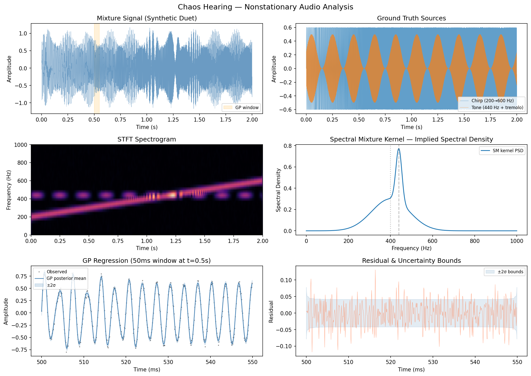
Top: mixture signal and ground truth sources. Middle: STFT spectrogram vs. spectral mixture kernel density. Bottom: GP posterior mean and uncertainty on a 50ms window.
EP via Kalman Smoothing (Algorithm 1)
Implementation of Algorithm 1 from Wilkinson et al. (2019) — Expectation Propagation inference in a state-space GP model via Kalman filtering (forward pass) and RTS smoothing (backward pass).
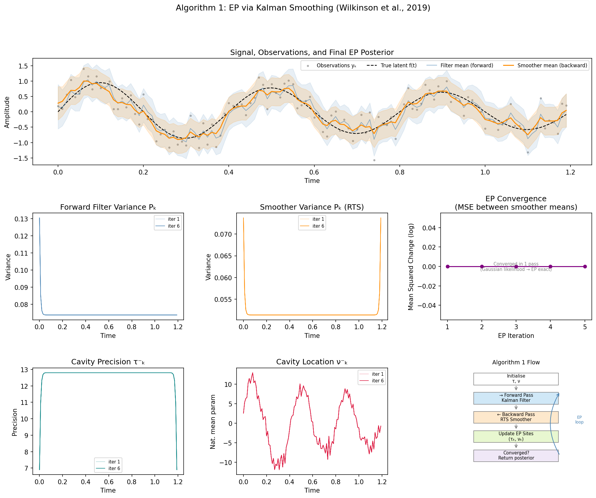
Top: observations, true latent signal, and final EP posterior (filter in blue, smoother in orange). Middle: variance evolution across EP iterations and convergence. Bottom: cavity parameters τ⁻ and ν⁻ stabilising, plus algorithm flow diagram.
The smoother consistently outperforms the filter (RMSE ~0.16 vs ~0.21) because it incorporates future observations — the backward pass propagates information from the end of the signal back to the beginning.